
 Navigate to your Google Drive account. You can find this by opening a new tab in Chrome and if you’re already logged in, then there should be a grid button next to your profile on the top right. If not, sign in first then you can navigate to this button. It will bring up all the options available including Google Drive which is the triangular icon with a triangular hole in the middle.
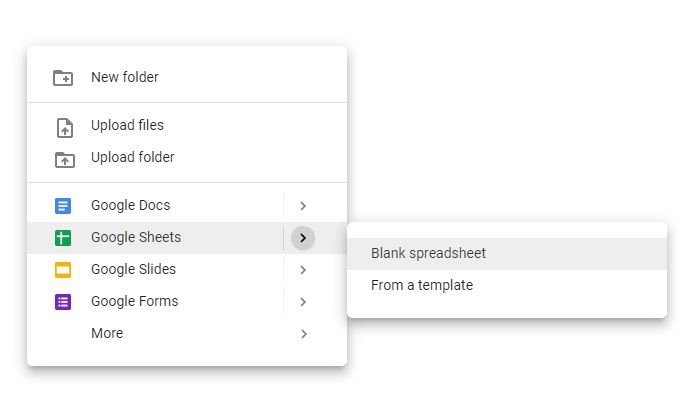
On your drive, you can right click anywhere and a menu will show up. Scroll down to Google Sheets and create a New Spreadsheet.
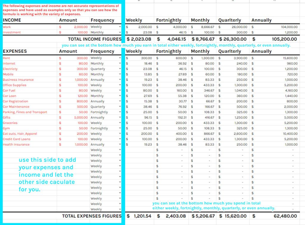
To see your expenses into perspective, you’d want to see how much it accumulates Weekly, Fortnightly, Monthly, Quarterly, and Annually. We would need a column for each of these, plus a column for the description. However, to make it easier for us later, we will have two additional columns: Amount and Frequency.
These two will be placed just after the Description but before the rest of the columns.

What does this do? Different things are billed at different cycles. You might have your phone bill billed monthly but your rent is billed weekly. This helps automate our calculations in the long run and save us some time. We will make the Frequency column a dropdown option for Weekly, Fortnightly, Monthly, Quarterly, and Annually. Then depending on these options, this will calculate automatically how much the expense is for the other columns.
 To create our frequency dropdown, select the cell that is immediately underneath the title word “Frequency”.
While you have it selected, Go to the Menu > Data > Data Validation.
This will bring up a pop up with a few options. In the pop up, pick List of Items and tick the Show Dropdown list in cell. In the texbox type:
Weekly,Fortnightly,Monthly,Quarterly,Annually
The commas separate each option. Then click Save.

The next colums are a little trickier. We will start with the Weekly column. We want to make a statement that if the dropdown in the frequency column says weekly, then the amount next to it will be reflected, otherwise:
- if it says fortnightly then we will have to divide it by 2 to get a weekly amount.
- if it says monthly then we will have to multiply it by 12 and divide it by 52 to get a weekly amount.
- if it says quarterly then we will have to multiply it by 4 then divide it by 52 to get a weekly amount.
- if it says annually then we will have to divide it by 52 to get a weekly amount.
This is a massive IF statement formula which looks like this:
=if(C2=“Weekly”,B2,if(C2=“Fortnightly”,B2/2,if(C2=“Monthly”,(B2*12)/52,if(C2=“Quarterly”,B2/13,if(C2=“Annually”,B2/52,0)))))
Basically you need to make sure you’re not missing a bracket.
Instead of repeating the formula each time and painstakingly changing the cells, you can drag the formulas down and it will automatically adjust.
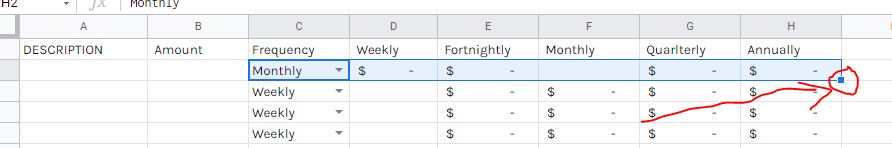
Drag it down at least 10 times as you probably have this many (or more) expenses.
At the bottom of all your expenses, we need a row that shows us the total expenses. These should add up all the data above.

We can’t total the Amount as it varies from weekly to monthly, etc. We also can not total the frequency. However, we can total the Weekly, Fortnightly, Monthly, Quarterly, and Annually columns. This helps us see how much our expenses cost all together; whether it is weekly, fortnightly, monthly, quarterly, or annually.
To add everything in a column, you can write the formula:
=SUM(firstcell:lastcell)
As long as the data is all lined up in one column. Example for the image above:
=sum(D2:D30)
My expenses run until the 30th column so my last cell is D30.

Jozzelle De Jesus
Multimedia Designer
Jozzelle has been working professionally in the graphic design area since 2006 and tackled freelance design and animation since 2011. She has acquired a Bachelor of Interactive Entertainment (Animation) back in 2012 and completed a Cert IV in Training and Assessment in 2013. These days, she teaches graphic design with RTO's whilst she continues her work with current clients. If you would like to work with Jozzelle, please email hello@e-studios.com.au